Introduction to intersection modeling
This section provides an overview to intersection modeling. Topics include:
Why use intersection modeling?
In a traditional capacity restrained transport planning model, the effects of congestion are represented by link cost functions that assign costs to each link as a monotonic non-decreasing function of the flow on that link. This form of model has a unique Wardrop equilibrium solution. Furthermore, the Frank-Wolfe algorithm (invoked by default in CUBE Voyager) gives us a reasonably good solution algorithm. Thus later in the planning process, when we wish to compare schemes, we can be sure that, provided both models have been run to an adequate level of convergence, we have stable comparable results. Furthermore we can achieve good convergence in reasonable time.
Models with separable costs and monotonic non-decreasing cost functions have been very successful in modelling interurban travel. They have been applied to most kinds of geographic region and most kinds of planning decision.
However, in congested urban environments, it can easily be observed that most of the delay arises from the conflicts between streams at intersections. In such a situation, it may be necessary to use non-separable cost functions to achieve adequate verisimilitude in the sensitivities of the costs to the flows. Furthermore, if the policy responses being evaluated include traffic management measures (for example, changing the form of control at key intersections) it must be possible to represent the proposals in the model.
How the intersection models work
CUBE Voyager intersection modelling occurs during the ADJUST phase of a capacity restrained assignment. Data from a file of "Junction Descriptions" is read to determine the exact model form for each modelled node. When the costs arising from a flow pattern are required, the flow pattern is passed to the intersection model. The model will allocate the turning movements (which can be defined by the TURNS command) into lane groups, with each lane group having a capacity. Note that the capacity of a lane group will be reduced by any conflicting flows through the intersection. A delay function is applied to calculate the average delay per vehicle for vehicles in the lane group. These calculated delays are then applied as turn penalties in the next path build.
Limitations of intersection modeling
As noted above, intersection modelling tends to make the overall network model less stable. Consequently the assignment may take many more iterations to converge. Indeed, using the default method of combination, the model may never reach adequate levels of convergence. If necessary, you can change to using COMBINE=AVE to guarantee eventual convergence.
Note: A global minimum capacity of 1 vehicle (or PCU) per hour is now enforced. A PCU is similar to a vehicle but it is adjusted for vehicle length, so a car counts 1, a bus counts 2. Trucks vary between 1.5 (light van) and 2.5 (tractor-trailer).
CUBE Voyager intersection modelling and other programs
This chapter describes only those junction description keywords that are directly relevant to CUBE Voyager intersection modelling. However there are several other keywords permitted in an intersection description. Some of these extra keywords are used by CUBE graphics to assist in editing and display of intersections. Some of these extra keywords are used to preserve data that is required or used by CUBE Dynasim.
Methodology for U-Turns at Signalized Intersections
The methodology for modeling U-turn is to compute a HCM like saturation flow adjustment factor for U-turns and include it as a factor in the HCM computation for the U-turn lane group (either shared or exclusive).
A shared u-turn movement is generally allowed from the left turn lane or from the left most, left turn lane if the intersection has more than one left turn lane. A shared lane here means that either movement (left or u-turn) may be made from the same lane. Some intersections configurations also provide an exclusive u-turn lane in addition to one or more exclusive left turn lanes. When a u-turn movement is allowed from a shared left turn lane the increasing proportion of the u-turning flow can affect the overall capacity of the movement. This reduction in capacity is estimated by applying an adjustment factor.
The HCM determination of Saturation Flow Rate (S) is a function of a base flow rate (generally assumed to be 1900 vph/ln) times the number of lanes and then factored by various adjustment factors Fi based on prevailing conditions at the approach under consideration. The proposed methodology introduces an additional adjustment factor specifically for a u-turn movement. A simplified formulation for saturation flow rate is:
(1)
where,
-
S0 = base flow rate (assumed to be 1900 vph/ln) N = number of lanes for U-turn movement
-
Fi = various adjustment factors based on prevailing conditions at the approach for U-turn from HCM2000
-
Fut = U-turn adjustment factor based on estimates from Carter, D. et al. TRR 1912, 2005.
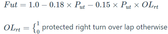
In implementation the user can provide the relationship between U-turn flow proportion and U-turn Adjustment Factor based on their own observed data if available via a U-turn slope parameter
(Fus) such that:
Otherwise u-turn slope parameter (Fus) would take on a default values base on the relationships estimated by Carter, D et al.
The table below provides an example of the effects of
increasing u- turn flow proportion on the saturation flow rate of a shared
left/u- turn lane. In this example we use the default u-turn slope parameter of
0.18 and assume that there is no right turn overlap condition (as that is
likely to be the case for all intersections in the current Abu Dhabi network).
The proportion of u-turn flow is then the ratio of u-turn flow to approach
flow, the u-turn adjustment factor
![]() and
and
![]() . When the u-turn flow proportion
is 1.0 the lane is effectively an exclusive u-turn lane with an adjustment
factor of 0.82.
. When the u-turn flow proportion
is 1.0 the lane is effectively an exclusive u-turn lane with an adjustment
factor of 0.82.
Effect of U-turn flow on lane Saturation Flow Rate S
| Left Flow | U-turn flow | Approach flow | Put | Fut | S |
|---|---|---|---|---|---|
| 1000 | 0 | 1000 | 0.0000 | 1.0000 | 1900 |
| 900 | 100 | 1000 | 0.1000 | 0.9820 | 1866 |
| 800 | 200 | 1000 | 0.2000 | 0.9640 | 1832 |
| 700 | 300 | 1000 | 0.3000 | 0.9460 | 1797 |
| 600 | 400 | 1000 | 0.4000 | 0.9280 | 1763 |
| 500 | 500 | 1000 | 0.5000 | 0.9100 | 1729 |
| 400 | 600 | 1000 | 0.6000 | 0.8920 | 1695 |
| 300 | 700 | 1000 | 0.7000 | 0.8740 | 1661 |
| 200 | 800 | 1000 | 0.8000 | 0.8560 | 1626 |
| 100 | 900 | 1000 | 0.9000 | 0.8380 | 1592 |
| 0 | 1000 | 1000 | 1.0000 | 0.8200 | 1558 |
Methodology for Free Right Turns at Signalized Intersections
In general a free-right turn is a right turn movement at a controlled intersection whereby the use of a slip lane or channel lane, the right turn movement can be made without being subjected to the signal control - thus the term ‘free’ implying the movement is free of the signal delay effects. In the ideal case a free-right turn lane configuration would have adequate entry and exit lane lengths to minimize or eliminate delay associated with accessing the entry lane or merging from the exit lane thus rendering the delay associated with the movement negligible. In practice however, often this ideal case is not the case and entry and exit lane lengths vary across a range from non-existent to the full length of the block face. This is the case in the reality where the as built conditions can vary widely from one intersection configuration to another. The methodology for modeling free right turn is sensitive to this level of variability in as built conditions.
The flow capacity for the free right movement is determined by the limiting flow rate between the entry/deceleration lane and the exit/acceleration lane. If through flow queuing during the red phase blocks entrance to the deceleration lane this could be the limiting flow rate for the free right movement. However, limits due to yielding and/or merging due to conflicting traffic at the acceleration lane could also be the limiting flow rate.
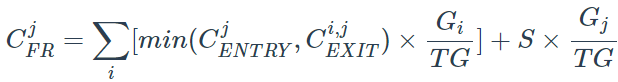
The flow capacity for the free right movement of a signalized intersection approach can then be defined as:
(2)
where,
CjFR = capacity of a free right movement for an approach j at a signalized intersection
CjENTRY= capacity based on entry into right turn deceleration lane during the red time for approach j
Ci,jEXIT = capacity based on exit from the right turn acceleration lane during the red time for approach j during signal phase i
S = saturation flow for the free right movement during the green phase as defined in HCM2000 equation 16-4
Gi = green time at phase i
Gj = green time for through movement at approach j (free right is protected)
TG = total green time for all signal phases at the intersection
Entry Capacity CjENTRY
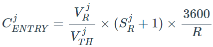
The entry lane capacity can be affected by the signal cycle if the queue length of the vehicles in the right most through lane during the red phase of the approach exceeds the length of the deceleration or slip lane. This entry lane limiting blocking capacity is based on the average maximum number of right lane vehicles served before through traffic blocks the entry into the right turn pocket/channel and can be computed as:
(3)
where,
SjR = number of vehicles (PCUs in STEAM model context) that can queue up in the right most through lane before it blocks the entry into the right turn pocket/channel (length of right turn storage bay in vehicles or distance from the stop line to the entry point to the right turn channel in vehicles if no right turn storage bay). This parameter value is computed from the user supplied length of the entry lane (Free Turn Entry Length) in meters (or feet if US units) and the average queued vehicle density (Queued Vehicle Spacing in meters/feet) specified by the users. Presence of some positive value for Free Turn Entry Length triggers the free right turn model to be applied for the right turn movement of the approach.
VjR = right turn volume at approach j (vph)
VjTH = volume in the right most through lane at approach j (vph)
(4)

where,
VjTOT = total volume in the through lane group at approach j (vph)
LjTOT = total number of lanes in the through lane group at approach j (vph)
fjLU = lane utilization factor at approach j from HCM2000 exhibit 10-23
This entry capacity is independent of the presence multiple lanes for the free right movement as it only depends on the through queue blocking entry.
Exit CapacityCi,jEXIT
A gap acceptance model for the determination of the flow rate at the exit would be appropriate for the case with little or no acceleration lane however some adjustment needs to be made to account for the length of the acceleration lane if one is present. As the length of the exit/acceleration lane increases the less impact there is on the lanes flow rate due to merging and lane changing with conflicting flow such that the flow rate should approach the saturation flow rate s, as defined in HCM2000.
The exit lane capacity for approach j during signal phase i can be defined as:
If EjL = 0 :
(5)

(6)
where,
EjL = length in meters (or feet) of the right turn exit/acceleration lane. This parameter is specified by the users. Measured from the first point a vehicle could enter the conflicting traffic stream to the last point a vehicle could enter the conflicting traffic stream.
EjMAX = maximum exit lane length. Lane lengths at or greater MAX than this value have no effect on capacity. This defaults to 160m but can be overridden by the user.
Ci,jGA = gap acceptance model based capacity computed as a signal time weighted average capacity computed for each interval of the signal cycle during the red phase for the approach. During the green phase of the approach the capacity is assumed to be at saturation flow (1900vph). Functional form uses TWSC gap acceptance model per HCM2000 equation 17-3 but with adjusted critical gap and follow-up time parameters:
(7)

where,
VjC = conflicting flow rate for the free right movement at approach j
tc = critical gap, i.e., the minimum time that allows vehicle for a free right movement. It’s a user-specified parameter with a default value of 4 seconds.
t_c_f = follow-up time, i.e., the time between the departure of one vehicle from approach and the departure of the next under a continuous queue condition. A user-specified parameter with a default value of 2.5 seconds.
Given the default values of critical gap and follow-up time, the above relationship to compute exit lane capacity based on a gap acceptance model adjusted for the length of the exit lane is depicted in the figure below:
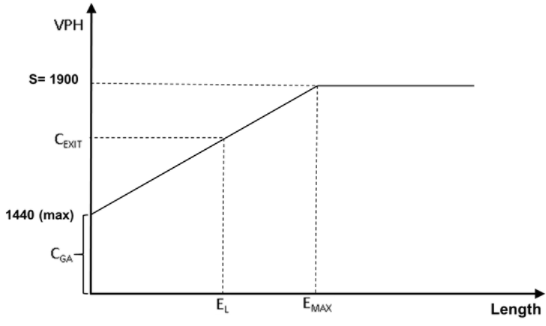
The upper limiting value of the capacity from the gap acceptance model is the value computed as the conflicting flow approaches zero and is a function of the assumed critical gap and follow up time parameters used. Based on the default values for these parameters this upper limiting value is 1440.
In cases where multiple lanes are present for the free right movement the number of lanes is included in the computation for the exit saturation flow. However a reduction factor should be applied similar to the method used for two lane entry to round about circulation lanes.
Once the entry and exit capacities are determined, \(C^j_{FR}\) determined and used to compute delay from a modified HCM Exhibit 17-38 formula as:
(8)

where,
CjFR = capacity of a free right movement for an approach j at a signalized intersection
T = analysis time period (h)
VjR = right turn volume at approach j (vph)